[Dynamic Programming] Policy Iteration
We will sequentially cover Dynamic Programming, Monte Carlo methods, and Temporal Difference methods. Sutton describes these methods in his book as follows:
“Dynamic programming, Monte Carlo methods, and temporal-difference learning. Each class of methods has its strengths and weaknesses. Dynamic programming methods are well developed mathematically, but require a complete and accurate model of the environment. Monte Carlo methods don’t require a model and are conceptually simple, but are not suited for step-by-step incremental computation. Finally, temporal-difference methods require no model and are fully incremental, but are more complex to analyze. The methods also differ in several ways with respect to their efficiency and speed of convergence.”
Sutton also defines Dynamic Programming as follows:
“The term dynamic programming (DP) refers to a collection of algorithms that can be used to compute optimal policies given a perfect model of the environment as a Markov decision process (MDP).”
Planning vs Learning
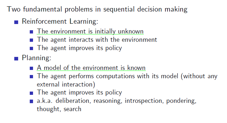
Before explaining Dynamic Programming in detail, let’s first look at the difference between Planning and Learning. Simply put:
- Planning refers to solving problems with knowledge of the environment’s model.
- Learning refers to solving problems without knowing the environment’s model, but by interacting with it.
Dynamic Programming is a Planning method, assuming we know the environment’s model (reward, state transition matrix), and it solves problems using the Bellman equation. Although Planning and Learning are distinct in Reinforcement Learning, understanding DP is crucial since RL evolved based on DP principles.
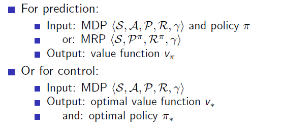
Prediction & Control
Dynamic Programming consists of two main steps: (1) Prediction and (2) Control. These steps help us understand how DP operates:
- Prediction: Calculate the value function for a given, non-optimal policy.
- Control: Improve the policy based on the current value function, and repeat this process to eventually find the optimal policy.
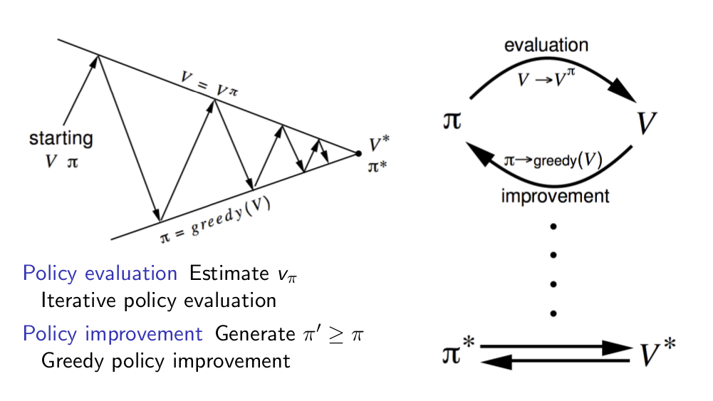
Policy Evaluation
Policy Evaluation is the process of solving the prediction problem: finding the true value function for a given policy using the Bellman equation. This involves iteratively updating the value function for all states simultaneously, using rewards and next states’ values.
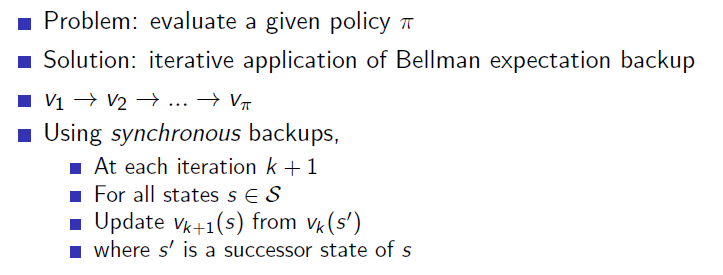
Below is the Bellman equation with the iteration count (k) to indicate the number of updates.
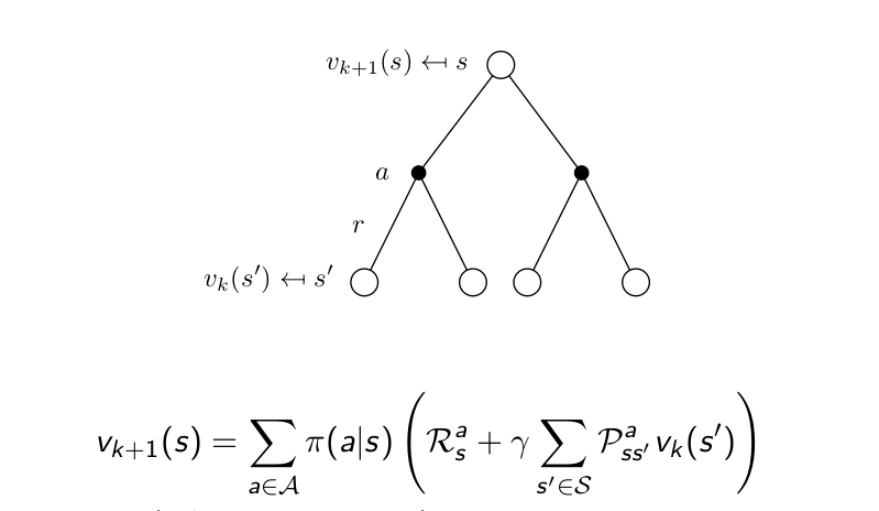
By calculating the Bellman equation for each state at each iteration, we gradually update the value function. This process continues until the value function converges for all states.
Gridworld Example
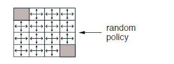
Consider the classic 4x4 gridworld example. This grid has two terminal states (gray), with 14 non-terminal states. The agent can take four actions: up, down, left, and right. Each time step gives a reward of -1, so the agent’s goal is to reach a terminal state as quickly as possible.

The process of finding the optimal policy involves two steps:
- Evaluation: Assess the current policy by computing the value function for each state.
- Improvement: Adjust the policy to improve it based on the value function.
Initially, we start with a uniform random policy where the agent moves randomly in all directions with equal probability. Let’s calculate the value function for this policy.
Value Function Update
In each iteration, we update the value function for each state using the Bellman equation:

For example:
- After the first iteration ((k=1)), the value of non-terminal states is calculated as
.
- After the second iteration ((k=2)), the value for state (1,2) is calculated as:
Here, the agent hits a wall when moving up, returning to the current state, resulting in updated value functions for the surrounding states. This iterative process continues until the value function converges for the current policy.
Policy Iteration
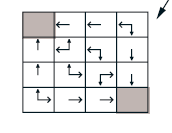
Once the value function is computed for the current policy, we move to Policy Improvement, where we update the policy based on the value function. The method used here is greedy improvement, which involves selecting the action that leads to the state with the highest value.
After the first round of improvement, the policy is updated to a more optimal one:
For small environments like this gridworld, a single round of policy evaluation and improvement can yield the optimal policy. However, in larger environments, this process often needs to be repeated multiple times, a process known as Policy Iteration.
Note that it is not always necessary to perform a full evaluation at each step. Sometimes, even a few iterations of policy evaluation can be enough to converge to the optimal policy.
Example Code
import numpy as np
import matplotlib.pyplot as plt
from matplotlib import animation
import logging

# 로깅 설정
logging.basicConfig(level=logging.INFO, format='%(message)s')

class PolicyIteration:
    def __init__(self, n_rows, n_cols, goal_point, gamma=0.9, theta=1e-6):
        self.n_rows = n_rows
        self.n_cols = n_cols
        self.n_states = n_rows * n_cols
        self.actions = ['up', 'down', 'left', 'right']
        self.gamma = gamma
        self.theta = theta
        self.v = np.zeros(self.n_states)
        self.policy = np.ones((self.n_states, len(self.actions))) / len(self.actions)  # 랜덤 정책으로 초기화 (각 행동에 대해 동일한 확률)  # 랜덤 정책으로 초기화
        self.goal_point = goal_point
        self.frames = []
        self.iteration_counts = []
        self.convergence_flags = []
        self.policies = [self.policy.copy()]  # 초기 정책을 저장

    def transition_reward(self, state, action):
        row, col = divmod(state, self.n_cols)
        if action == 'up':
            next_row, next_col = max(row - 1, 0), col
        elif action == 'down':
            next_row, next_col = min(row + 1, self.n_rows - 1), col
        elif action == 'left':
            next_row, next_col = row, max(col - 1, 0)
        elif action == 'right':
            next_row, next_col = row, min(col + 1, self.n_cols - 1)

        next_state = next_row * self.n_cols + next_col
        reward = 1 if next_state == self.goal_point else -1
        return next_state, reward

    def policy_evaluation(self):
        print("policy_evaluation")
        while True:
            delta = 0
            v_new_states = np.zeros(self.n_states)
            for state in range(self.n_states):
                v_new = 0
                for action_idx, action_prob in enumerate(self.policy[state]):  # 각 상태에서 모든 행동에 대한 기대 가치 계산
                    next_state, reward = self.transition_reward(state, self.actions[action_idx])
                    v_new += action_prob * (reward + self.gamma * self.v[next_state])
                delta = max(delta, abs(v_new - self.v[state]))  # 가치 함수의 변화량 추적
                v_new_states[state] = v_new
            self.v[:] = v_new_states[:]

            self.frames.append(self.v.copy())
            self.iteration_counts.append(len(self.iteration_counts))
            self.convergence_flags.append(delta < self.theta)

            if delta < self.theta:  # 가치 함수의 변화량이 기준치보다 작아지면 평가 종료
                break

    def policy_improvement(self):
        print("policy_improvement")

        # 새로운 개선된 정책을 저장하기 위한 배열을 초기화합니다.
        # 크기는 (상태의 수, 가능한 행동의 수)로 각 상태에서 각 행동을 선택할 확률을 나타냅니다.
        new_policy = np.zeros((self.n_states, len(self.actions)))

        # 각 상태(state)에 대해 정책을 개선합니다.
        for state in range(self.n_states):
            # 현재 상태에서 가능한 모든 행동의 가치를 계산하기 위해 리스트를 초기화합니다.
            action_values = []

            # 현재 상태에서 가능한 모든 행동(action)에 대해 반복합니다.
            for action in self.actions:
                # transition_reward 함수는 현재 상태와 행동을 받아서 다음 상태와 보상을 반환합니다.
                next_state, reward = self.transition_reward(state, action)

                # 행동 가치(action_value)를 계산합니다.
                # 행동 가치 = 현재 행동으로 얻는 보상 + 감가율(gamma) * 다음 상태의 가치
                # 다음 상태의 가치는 self.v[next_state]로 가져옵니다.
                action_value = reward + self.gamma * self.v[next_state]

                # 계산한 행동 가치를 action_values 리스트에 추가합니다.
                action_values.append(action_value)

            # 모든 가능한 행동 가치 중에서 가장 높은 가치를 갖는 행동의 인덱스를 찾습니다.
            # np.argmax(action_values)는 action_values 리스트에서 가장 큰 값을 가지는 인덱스를 반환합니다.
            best_action_idx = np.argmax(action_values)

            # 개선된 정책에서 현재 상태에서 가장 좋은 행동의 확률을 1로 설정합니다.
            # (즉, 가장 좋은 행동만을 선택하는 결정적 정책을 만듭니다.)
            new_policy[state][best_action_idx] = 1.0

        # 개선된 정책을 policies 리스트에 저장하여 정책 변화 과정을 추적할 수 있게 합니다.
        self.policies.append(new_policy)

        # 최종적으로 개선된 정책을 반환합니다.
        return new_policy

    def policy_iteration(self):
        while True:
            self.policy_evaluation()
            new_policy = self.policy_improvement()
            if np.allclose(new_policy, self.policy, atol=1e-3):  # 개선된 정책이 이전 정책과 거의 동일하면 반복 종료
                break
            self.policy = new_policy

    def animate(self):
        fig, ax = plt.subplots(figsize=(6, 6))

        def update(frame_idx):
            ax.clear()
            v = self.frames[frame_idx]
            iteration = self.iteration_counts[frame_idx]
            converged = self.convergence_flags[frame_idx]
            ax.imshow(v.reshape(self.n_rows, self.n_cols), cmap='coolwarm', interpolation='none', vmin=-20, vmax=1)
            ax.set_title(f'Iteration: {iteration} - Converged: {converged}, Destination{self.goal_point}')

            for i in range(self.n_rows):
                for j in range(self.n_cols):
                    state = i * self.n_cols + j
                    state_value = v[state]
                    ax.text(j, i, f'{state_value:.2f}', ha='center', va='center', color='black')
                    action_idx = np.argmax(self.policies[min(frame_idx, len(self.policies) - 1)][state])
                    action_str = ['↑', '↓', '←', '→'][action_idx]
                    ax.text(j, i + 0.3, f'{action_str}', ha='center', va='center', color='blue')

            ax.grid(False)
            ax.set_xticks([])
            ax.set_yticks([])

        ani = animation.FuncAnimation(fig, update, frames=len(self.frames), interval=300, repeat=False)
        plt.show()

if __name__ == '__main__':
    goal_point = int(input('goal_point 의 index를 정수로 입력하세요 : '))
    pi = PolicyIteration(n_rows=7, n_cols=7, goal_point=goal_point)
    pi.policy_iteration()
    pi.animate()
Leave a comment