[Monte Carlo] Monte Carlo Prediction

Model-Free Methods

In previous chapters, we learned about Dynamic Programming (DP). While DP is effective for solving MDPs with complete information about the environment, it has limitations:

1. Full-width Backup → expensive computation
2. Requires full knowledge about Environment

Monte Carlo methods differ from DP in two key aspects:

1. They learn from actual experience (sample episodes)
2. They don’t require complete knowledge of the environment

These limitations make DP impractical for complex real-world problems. Instead, we need methods that can learn from experience, similar to how humans learn through trial and error.

Instead of using full-width backup like DP, we perform sample backup using actual experienced information. By utilizing real experiences, we don’t need to know everything about the environment from the beginning. Since we learn without knowing the environment model, this approach is called “Model-free.”

When we update the value function through sampling based on the current policy, it’s called model-free prediction. If we also update the policy itself, it’s called model-free control.

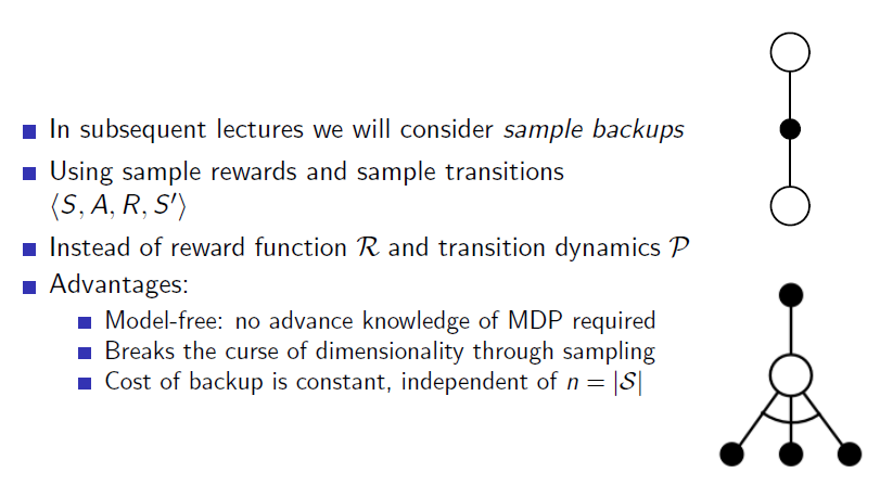
Sample backups use actual experience (S, A, R, S’) instead of complete MDP dynamics, making them more efficient and practical for real-world applications.

There are two main approaches to learning through sampling:

1. Monte Carlo
   • Updates after each episode
2. Temporal Difference
   • Updates after each time step

In this chapter, we’ll focus on Monte Carlo Learning.

---

Monte Carlo Methods

Sutton defines Monte Carlo methods as follows:

“The term ‘Monte Carlo’ is often used more broadly for any estimation method whose operation involves a significant random component. Here we use it specifically for methods based on averaging complete returns.”

The term “Monte Carlo” itself refers to measuring something randomly. In reinforcement learning, it means “averaging complete returns.” What does this mean?

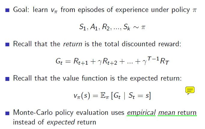
The distinction between Monte Carlo and Temporal Difference lies in the method of estimating the value function. The value function is the expected accumulative future reward, which is the total expected reward from the current state to the future. How can we measure this without using DP?

The most basic idea is to calculate the value functions of each state in reverse after experiencing the entire episode and receiving rewards. Therefore, MC (Monte Carlo) cannot be used for episodes that do not end. Starting from the initial state S1 to the terminal state St, if you follow the current policy, you will receive rewards at each time step. You remember those rewards, and when you reach St, you look back and calculate the value function of each state. Below, it says “recall that the return,” which is the same as what I mentioned. You can obtain the sample return by discounting the rewards received moment by moment in chronological order.

---

First-Visit vs Every-Visit MC

Earlier, we discussed what to do after an episode ends. But how do we calculate the return for each episode when dealing with multiple episodes? In MC, we simply take the average. If a return for a certain state is calculated in one episode and a new return is obtained for the same state in another episode, we average these two returns. As more returns accumulate, they converge closer to the true value function.

There is one consideration: what if a state is visited twice within a single episode? Depending on how this is handled, there are two approaches:

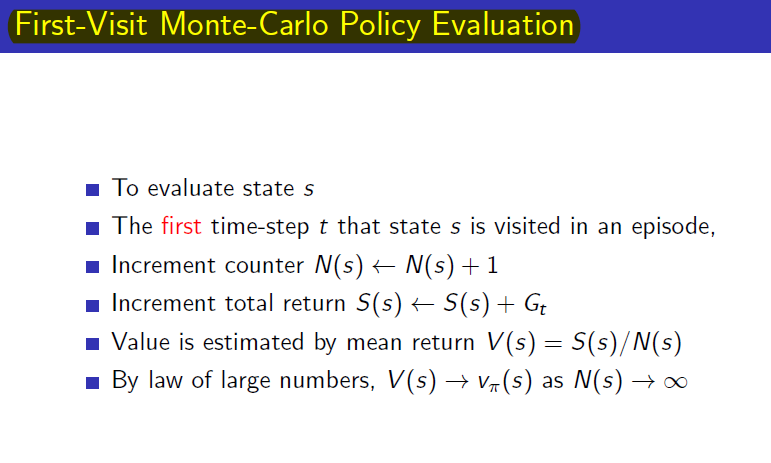
• First-visit Monte-Carlo Policy evaluation
• Every-visit Monte-Carlo Policy evaluation

As the names suggest, First-visit only considers the first visit to a state (ignoring returns for subsequent visits), while Every-visit calculates returns separately for each visit. Both methods converge to the true value function as the number of episodes approaches infinity. However, since First-visit has been more widely studied over a longer period, we will focus on First-visit MC here. Below is material from Professor Silver’s class on First-Visit Monte-Carlo Policy Evaluation.

---

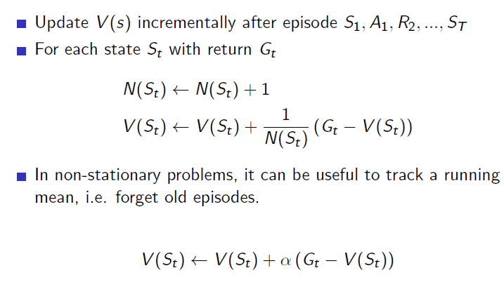
Incremental Mean

The formula for taking the average above can be further developed as follows. Instead of averaging all at once, we calculate the average incrementally, adding one by one, which can be expressed with the Incremental Mean formula below.

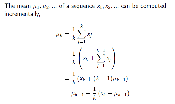
Applying this Incremental Mean to the First-visit MC above, we can express it differently as shown below. Here, as N(St) in the denominator approaches infinity, we can fix it as alpha to effectively take the average. This can be seen as giving less weight to the initial information. (Those familiar with the complementary filter will find this easier to understand.) The reason for doing this is that reinforcement learning is not a stationary problem. Since a new policy is used in each episode (we haven’t discussed policy updates yet), it is a non-stationary problem, so the constant used for updates is fixed.

---

Backup Diagram

이러한 MC의 backup과정을 그림으로 나타내면 아래과 같습니다.

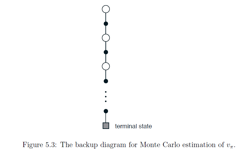
In the backup diagram of DP, only one step is shown, whereas in MC, it extends all the way to the terminal state. Additionally, in DP, the one-step backup branches out to all possible next states, but in MC, due to sampling, it follows a single path to the terminal state.

Monte Carlo was initially described as a method involving a random process, and because updates occur after each episode, the starting point and the direction taken at the same state (left or right) can lead to entirely different experiences. Due to these random elements, MC has high variance. However, since it is random, it tends to have less bias, as it is less likely to be skewed in any particular direction.

---