[Monte Carlo] Monte Carlo Control with Python code

Monte-Carlo Policy Iteration

Previously, we looked at Monte-Carlo Policy Evaluation = Prediction. Just as evaluation + Improvement = Policy Iteration in Dynamic Programming, in MC, Monte-Carlo Policy Evaluation + Policy Improvement becomes Monte-Carlo Policy Iteration.

Let’s revisit DP’s Policy Iteration. Based on the current policy, the value function is iteratively calculated to evaluate the policy (until it converges to the true value function), and then the policy is improved greedily based on that value function. This process is repeated until the optimal policy is obtained.

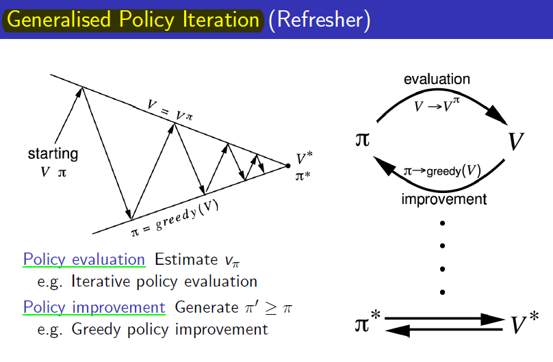
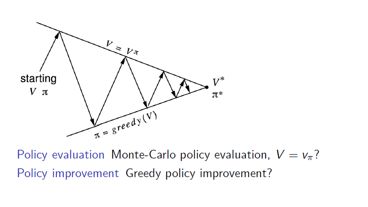
If we replace only the Policy evaluation with Monte-Carlo policy evaluation, it becomes Monte-Carlo Policy Iteration.

---

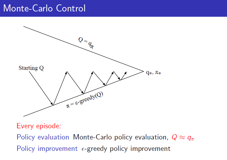
Monte-Carlo Control

However, there are three issues with Monte-Carlo Policy Iteration:

• Value function
• Exploration
• Policy Iteration

1. Value function

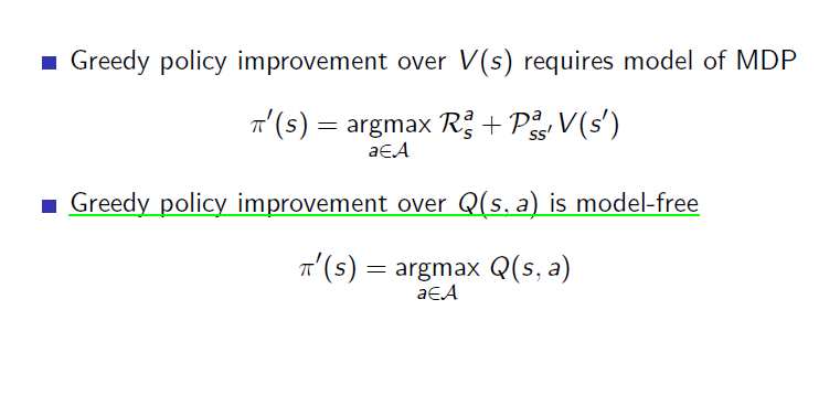
Currently, MC uses the Value function to evaluate the policy. However, using the value function causes problems when improving the policy (greedy). The original reason for using MC was to be Model-free, but to improve the policy with the value function, the MDP model must be known. To calculate the next policy as shown below, the reward and transition probability must be known. Therefore, instead of the value function, the action value function is used. This allows for model-free operation without such issues.

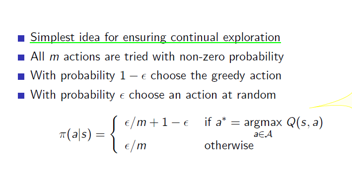
2. Exploration

Currently, policy improvement uses greedy policy improvement. However, if only the best option in the current situation is considered, it may not lead to the optimal solution but rather fall into a local optimum. This is because sufficient exploration was not conducted, preventing reaching the global optimum. If action a is measured to have the highest value function and only action a is taken, the possibility that action b might have a higher value function is excluded. It might be a mistake similar to selecting people based only on university or grades. Therefore, as an alternative, a certain probability is used to take a different action that does not have the highest value in the current state. This probability is called epsilon, and this improvement method is called epsilon greedy policy improvement. If there are m actions to choose from, the greedy action (the action with the highest action value function) and other actions are divided and selected with the probabilities shown below. This allows for the exploration that was previously lacking.

3. Policy Iteration

In Policy Iteration, the evaluation process must be done until it converges to the true value function, but it was said that even if policy improvement is done after one evaluation, it leads to the optimal solution. This was Value iteration, and similarly, by reducing the evaluation process in Monte-Carlo, Monte-Carlo policy iteration becomes Monte-Carlo Control. Ultimately, Monte-Carlo Control is as follows.

---

GLIE

GLIE stands for Greedy in the Limit with Infinite Exploration. Although it is not mentioned in Professor Sutton’s book, it was covered in Professor Silver’s lecture. It refers to converging to a greedy policy after sufficient exploration during learning. However, epsilon greedy policy does not select only one action greedily, so it is not GLIE in such cases. The optimal policy to be learned through learning is usually a greedy policy. Therefore, if epsilon in epsilon greedy, used due to exploration issues, converges to 0 over time, epsilon greedy can also become GLIE. Later, this issue is resolved by using Q-learning as off-policy control.

---

Example Code

import numpy as np
import matplotlib.pyplot as plt
from matplotlib import animation
import logging
import random

# 로깅 설정
logging.basicConfig(level=logging.INFO, format='%(message)s')

class MonteCarlo:
    def __init__(self, n_rows, n_cols, goal_point, gamma=0.9, episodes=1000, epsilon=0.1):
        # 1. 클래스 초기화
        self.n_rows = n_rows  # 격자의 행 수
        self.n_cols = n_cols  # 격자의 열 수
        self.n_states = n_rows * n_cols  # 상태의 총 수 (격자의 모든 칸)
        self.actions = ['up', 'down', 'left', 'right']  # 가능한 행동 리스트
        self.gamma = gamma  # 할인 계수 (감가율)
        self.goal_point = goal_point  # 목표 상태 설정
        self.v = np.zeros(self.n_states)  # 초기 가치 함수 설정 (모든 상태의 가치를 0으로 초기화)
        self.q = np.zeros((self.n_states, len(self.actions)))  # 행동 가치 함수 초기화
        self.returns = {(state, action): [] for state in range(self.n_states) for action in range(len(self.actions))}  # 각 상태-행동 쌍의 반환 값을 저장
        self.frames = []  # 애니메이션을 위한 가치 함수 저장 리스트
        self.iteration_counts = []  # 각 반복의 횟수를 저장
        self.episodes = episodes  # 에피소드 수 설정
        self.epsilon = epsilon  # 탐험(exploration) 확률 설정

    def transition_reward(self, state, action):
        # 4. 현재 상태와 행동에 따라 다음 상태와 보상을 계산
        row, col = divmod(state, self.n_cols)  # 현재 상태의 행과 열 계산
        
        # 행동에 따른 다음 상태 계산
        if action == 'up':
            next_row, next_col = max(row - 1, 0), col
        elif action == 'down':
            next_row, next_col = min(row + 1, self.n_rows - 1), col
        elif action == 'left':
            next_row, next_col = row, max(col - 1, 0)
        elif action == 'right':
            next_row, next_col = row, min(col + 1, self.n_cols - 1)
        
        next_state = next_row * self.n_cols + next_col  # 다음 상태의 인덱스 계산
        reward = 1 if next_state == self.goal_point else -1  # 목표 상태에 도달하면 +1, 그렇지 않으면 -1의 보상
        return next_state, reward

    def choose_action(self, state):
        # 3. epsilon-greedy 정책을 사용하여 행동 선택
        if random.uniform(0, 1) < self.epsilon:
            return random.randint(0, len(self.actions) - 1)  # 탐험: 임의의 행동 선택
        else:
            return np.argmax(self.q[state])  # 착취: 최대 행동 가치 함수를 가지는 행동 선택

    def generate_episode(self):
        # 에피소드 생성: 초기 상태에서 목표 상태까지의 경로를 생성
        episode = []  # (state, action, reward) 튜플을 저장할 리스트
        state = random.randint(0, self.n_states - 1)  # 임의의 초기 상태 선택
        
        while state != self.goal_point:
            action = self.choose_action(state)  # epsilon-greedy 정책에 따라 행동 선택
            next_state, reward = self.transition_reward(state, self.actions[action])
            episode.append((state, action, reward))  # 현재 상태, 행동, 보상을 에피소드에 추가
            state = next_state  # 다음 상태로 이동
        
        return episode

    def monte_carlo_control(self):
        # Monte Carlo Control 알고리즘 실행
        print("monte_carlo_control")
        for episode_idx in range(self.episodes):
            episode = self.generate_episode()  # 에피소드 생성
            g = 0  # 반환 값 초기화
            visited_state_action_pairs = set()  # 방문한 상태-행동 쌍 저장
            
            # 에피소드의 각 상태-행동에 대해 반환 값을 계산하고 행동 가치 함수 갱신
            for state, action, reward in reversed(episode):
                g = reward + self.gamma * g  # 반환 값 갱신
                if (state, action) not in visited_state_action_pairs:  # 첫 방문 여부 확인
                    visited_state_action_pairs.add((state, action))
                    self.returns[(state, action)].append(g)  # 반환 값을 저장
                    self.q[state, action] = np.mean(self.returns[(state, action)])  # 상태-행동 가치 함수 갱신
                    
                    # 가치 함수 갱신: 각 상태에서 가능한 행동 중 최대 가치 선택
                    self.v[state] = np.max(self.q[state])
            
            # 애니메이션 프레임 저장
            self.frames.append(self.v.copy())
            self.iteration_counts.append(episode_idx)

    def animate(self):
        # 애니메이션 생성: 각 에피소드 후의 상태 가치 함수를 시각화
        fig, ax = plt.subplots(figsize=(6, 6))

        def update(frame_idx):
            ax.clear()
            v = self.frames[frame_idx]
            iteration = self.iteration_counts[frame_idx]
            ax.imshow(v.reshape(self.n_rows, self.n_cols), cmap='coolwarm', interpolation='none', vmin=-20, vmax=1)
            ax.set_title(f'Episode: {iteration}, Destination: {self.goal_point}')

            for i in range(self.n_rows):
                for j in range(self.n_cols):
                    state = i * self.n_cols + j
                    state_value = v[state]
                    ax.text(j, i, f'{state_value:.2f}', ha='center', va='center', color='black')

            ax.grid(False)
            ax.set_xticks([])
            ax.set_yticks([])

        ani = animation.FuncAnimation(fig, update, frames=len(self.frames), interval=300, repeat=False)
        plt.show()

if __name__ == '__main__':
    # 프로그램 시작: 목표 상태를 입력받고 Monte Carlo Control 실행
    goal_point = int(input('goal_point 의 index를 정수로 입력하세요 : '))
    mc = MonteCarlo(n_rows=7, n_cols=7, goal_point=goal_point)
    mc.monte_carlo_control()  # Monte Carlo Control 알고리즘 실행
    mc.animate()  # 결과 애니메이션

---